A Facile Calibration Method for Granular Materials

(This study is at the final stage of submission. Therefore, I cannot share more specific details of this study until my paper is published. However, after submission, I will share the entire manuscript of the paper.)

Introduction

Granular materials are widely used in various fields such as sintering, tablet manufacturing, and geotechnical engineering.

To predict their constitutive behavior in the finite element method (FEM), the modified Drucker–Prager Cap model (DPC model) is commonly adopted.

However, the conventional method requires multiple triaxial compression experiments and isotropic compression experiments to determine a great number of parameters in the DPC model.

This study proposes an alternative method for the DPC model that utilizes the entire stress–strain curves from triaxial compression tests and the gradient descent algorithm to extract the parameters.
The method significantly reduced the total optimization time by replacing FEM simulation with analytical calculations during the optimization process.

The method was applied to acquire the constitutive relation for unsaturated sand-bentonite mixtures, and it successfully predicted experimental depth-sensing indentation results using FEM simulation.

Theoretical Approach

Figure 1. Overall Algorithm

Fig. 1 describes the overall methodology used in this study.

In the beginning, the parameters are randomly selected.
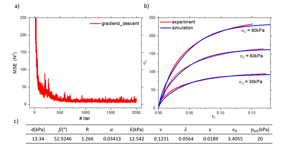
After selecting random parameters, the analytical expression calculates the stress–strain curve—the result of the triaxial compression test—from the selected parameters.
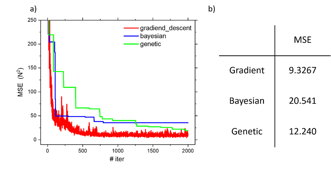
Afterward, the error between the experiment results and the calculation is computed. This study used mean squared error (MSE).
If MSE is larger than an objective value, the gradient descent algorithm updates the parameters and repeats the whole process until MSE becomes lower than the objective value.

Result and Discussion

Figure 2. Result of optimization. (a) mean square error during the optimization (b) fitted curve at the last stage of the optimization (c) optimized parameters

Fig. 2 is a result of optimization using the customized algorithm displayed in Fig. 1.

Fig. 2(a) shows the changes of MSE during the iterations. MSE converged after 500 iterations, and the final value was less than 10. It means that the difference between the experiment and the simulation is about 3 N, so it can be inferred that the DPC model parameters were calibrated with high precision.

Next, Fig. 2(b) compares the final curve to the triaxial compression test result. The red line is the experiment result, and the blue line is the calculated curve from the calibrated parameters. As mentioned above, the two curves were well matched to each other.

Finally, Fig. 2(c) shows the parameters fitted by the algorithm.

Table 1. Mean (\(\mu\)) and standard deviation (\(\sigma\) ) of the optimized DPC model parameters.

Table. 1 shows the mean and the standard deviation of the DPC model parameters calibrated from ten different initial points.
As indicated in the table, most of the parameters did not show significant variances.
It means that the triaxial compression test and the gradient descent algorithm were sufficient to characterize these parameters.

Figure 3. Load–depth curve of the indentation test and corresponding result of FE simulation which was implemented with the parameters obtained by the gradient descent algorithm.

The parameters shown in Fig. 2(c) were optimized to reproduce the triaxial compression test result.
Hence, we need to check whether the parameters are valid in other circumstances.
This study used an indentation test to substantiate the parameters’ validity.

Fig. 3 compares the result of the indentation test and its FE simulation result, which was implemented with the optimized parameters.
The indentation test was repeated nine times, and the blue line is the mean value of the experiment result.
The red line is the result of the FE simulation with the parameters shown in Fig. 2(c).

The entire red line is inside the error bar of the blue line. This result means that the parameters fitted from the triaxial compression test results can describe the constitutive behavior of the material in the general case.

Figure 4. Optimization result of gradient descent algorithm, Bayesian optimization, and genetic algorithm. (a) MSE vs iteration (b) final MSE

The analytical solution proposed in this study enabled the gradient descent algorithm to use because error gradients were computed from the solution. (We can not compute the gradients from FEM simulation!)
Here, the result of the gradient descent algorithm to that of Bayesian optimization (BO) and genetic algorithm (GA) to check the performances of the gradient descent algorithm. (BO and GA are representative derivative-free optimization method)

Fig. 4 compares the results of each optimization algorithm.
First, Fig. 4(a) shows the MSE changes during the optimization process. According to the figure, the gradient descent algorithm decreased the MSE faster than other algorithms did.
Second, Fig. 4(b) shows the final MSE of each optimization method. In Fig. 4(b), the final MSE of the gradient descent algorithm was lower than that of other algorithms.
In summary, the gradient descent algorithm was able to obtain more precise DPC model parameters in fewer iterations than derivative-free optimization algorithms.

Figure 5. Load-depth curves of the indentation test and FE simulation results with the parameters optimized by different algorithm.

Fig. 5 compares FE simulation results to the indentation experiment result. Each FE simulation was implemented with the DPC model parameters calibrated by different methods.

FE simulation with the parameters optimized by BO falls outside the error range of the experiment in the early displacement region. This was because the parameters fitted by BO showed bigger MSE than the parameters evaluated by the gradient descent algorithm. (Fig. 4(b))

The parameters fitted with the GA caused a significant deviation from the experiment results in the FE simulation. The updating rules of the method may have caused this massive error. In a GA, parameters having considerable deviation in small domains may survive in a generation if the overall MSE is lower than others. Therefore, the parameters that only affect small domains may not be fitted correctly by this algorithm.

Conclusion

This study developed a novel characterization method by utilizing the triaxial compression test, the algorithm that calculates the material's constitutive behavior during the triaxial compression test, and the gradient descent algorithm.
The proposed method was possible because the triaxial compression test results contain information about shearing and hardening.
The algorithm for the constitutive behavior of the material replaced the time-consuming FE simulation in the optimization process, so the total optimization time decreased.
In addition, the algorithm made it possible to use the gradient descent algorithm to calibrate the DPC model parameters.

The gradient descent algorithm converged faster and produced more precise parameters than Bayesian optimization and genetic algorithm.
The fitted parameters can be used in general circumstances, as we confirmed in the indentation experiment.
From this study, we expect that people may characterize any granular materials more easily than before.
Also, the study may contribute to applying granular materials to fields that require high accuracies, such as micro-transfer printing or nanotechnology.